Every forward pass of a transformer activates every parameter. Ask something trivial or ask something hard - the whole network runs regardless. Scale up and compute scales with it, linearly. That gets expensive fast.
Mixture of Experts (MoE) breaks that. Each transformer block gets a pool of smaller expert networks and a router that chooses between them. Total parameters go up; per-token compute stays roughly constant. That's how DeepSeek-V4 fits 1.6T parameters while activating only 49B per token.
In this post I build one from scratch - the routing, dispatch logic and load-balancing loss - then compare it against a dense baseline. This is a deliberately small-scale experiment — the goal is mechanics, not benchmarks.
What is a Mixture of Experts (MoE)?
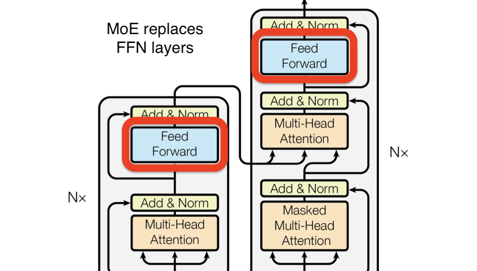
MoEs replace the feedforward layers in a transformer with a pool of smaller expert networks and a router that picks an expert per token.
A common misconception is that an MoE is a bunch of domain specialists wearing different hats (like a poet, journalist or scientist). The reality is much more granular. Rather than a "poetry expert", you might have an expert that is a specialist in punctuation or another that handles verb conjugation in specific contexts.
How the "Experts" Actually Work
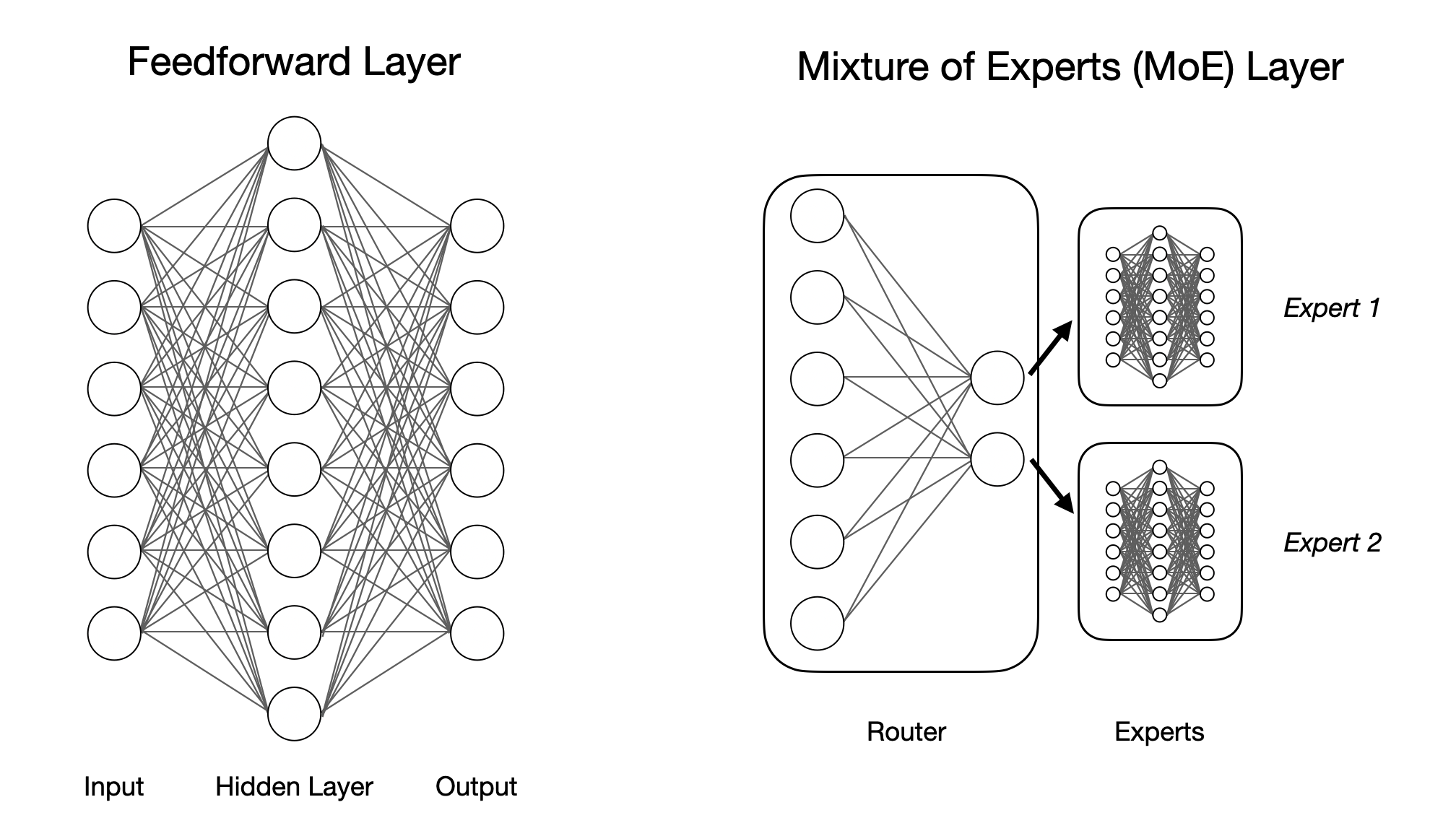
Each MoE block contains:
- Router: a small learnable layer that takes each token's input vector and picks its best-matched expert.
- Experts: standard feedforward networks (FFNs), each with their own unique weights.
Because only a few experts fire per token, the model can hold far more total parameters than a dense model at the same compute cost. That's the scaling trick.
The Anatomy of a Minimal MoE Block
To implement this from scratch, I need to handle the specific mechanical "plumbing" that happens inside an MoE block. Even in its simplest form, a single MoE block follows a strict sequence:
1. The Router
The input vector ("hidden state" from the previous layer) is multiplied by a learnable weight matrix to produce scores for each expert. A Softmax is applied to these scores to turn them into probabilities.
router = nn.Linear(d_model, num_experts)
Consider the following input to an MoE block:
# x shape = [batch, seq_len, d_model] = [2, 5, 8]
# 10 tokens total, each token is an 8-dim vector.

x = torch.tensor([
    [  # batch 0
        [ 0.2, -0.1, 0.0, 0.4, 0.1, -0.3, 0.5, 0.2],  # t0
        [ 0.0,  0.3, 0.2, 0.1,-0.2,  0.4, 0.1,-0.1],  # t1
        [ 0.5,  0.2,-0.4, 0.0, 0.3,  0.1,-0.2, 0.2],  # t2
        [-0.1, 0.1, 0.3, 0.2, 0.0, -0.2, 0.4, 0.1],  # t3
        [ 0.3, -0.2, 0.1, 0.5,-0.1,  0.0, 0.2, 0.3],  # t4
    ],
    [  # batch 1
        [ 0.1, 0.0,-0.2, 0.3, 0.4,  0.2,-0.1, 0.0],  # t0
        [-0.3,0.2, 0.1, 0.0, 0.2, -0.1, 0.3, 0.4],  # t1
        [ 0.4,0.1, 0.0,-0.2, 0.1,  0.3, 0.2,-0.1],  # t2
        [ 0.2,-0.4,0.3, 0.1, 0.0,  0.2,-0.2, 0.5],  # t3
        [ 0.0,0.2,-0.1, 0.4, 0.3, -0.3, 0.1, 0.2],  # t4
    ]
], dtype=torch.float32)

x_flat = x.reshape(10, 8)  # [B*T, D]
With 2 experts, the router output looks like:
num_experts = 2
probs = router(x_flat)

# A probability per token for each expert

probs = torch.tensor([
    [0.80, 0.20],  # batch 0, t0 has an 80% chance of being better suited to Expert 0
    [0.35, 0.65],
    [0.60, 0.40],
    [0.10, 0.90],
    [0.55, 0.45],
    [0.25, 0.75],
    [0.70, 0.30],
    [0.40, 0.60],
    [0.85, 0.15],
    [0.52, 0.48],
])  # shape [10, 2]
2. Top-k Selection
Once I have probabilities for each expert, I have to choose which expert does the work. There are two ways to do this:
Top-1 Routing: Pick only the single highest probability expert. This is the most efficient and is great for a minimal implementation. This is the approach I'll focus on.
Top-k Routing: Many production models pick the top k experts (like Mixtral 8x22B which does top-2), delegate to these and sum their outputs, weighted by router probability. This can help with training stability.
# Pick argmax expert per token
top1_idx = torch.argmax(probs, dim=-1)

# Example result:
top1_idx = torch.tensor([0, 1, 0, 1, 0, 1, 0, 1, 0, 0])  # shape [10]
# token 0 -> Expert 0, 1 -> Expert 1, 2 -> Expert 0, ...
One subtlety worth noting: argmax is non-differentiable, so the routing decision itself can't receive gradients. A standard extension is to weight
expert outputs by their router probability, giving the router a direct gradient path through the main loss - this implementation keeps it simple and
relies on the balancing loss instead (covered shortly here).
3. Dispatch & Combine
MoE blocks receive a batch of tokens, which must be split with each token routed through its selected expert, and then the tokens reassembled.
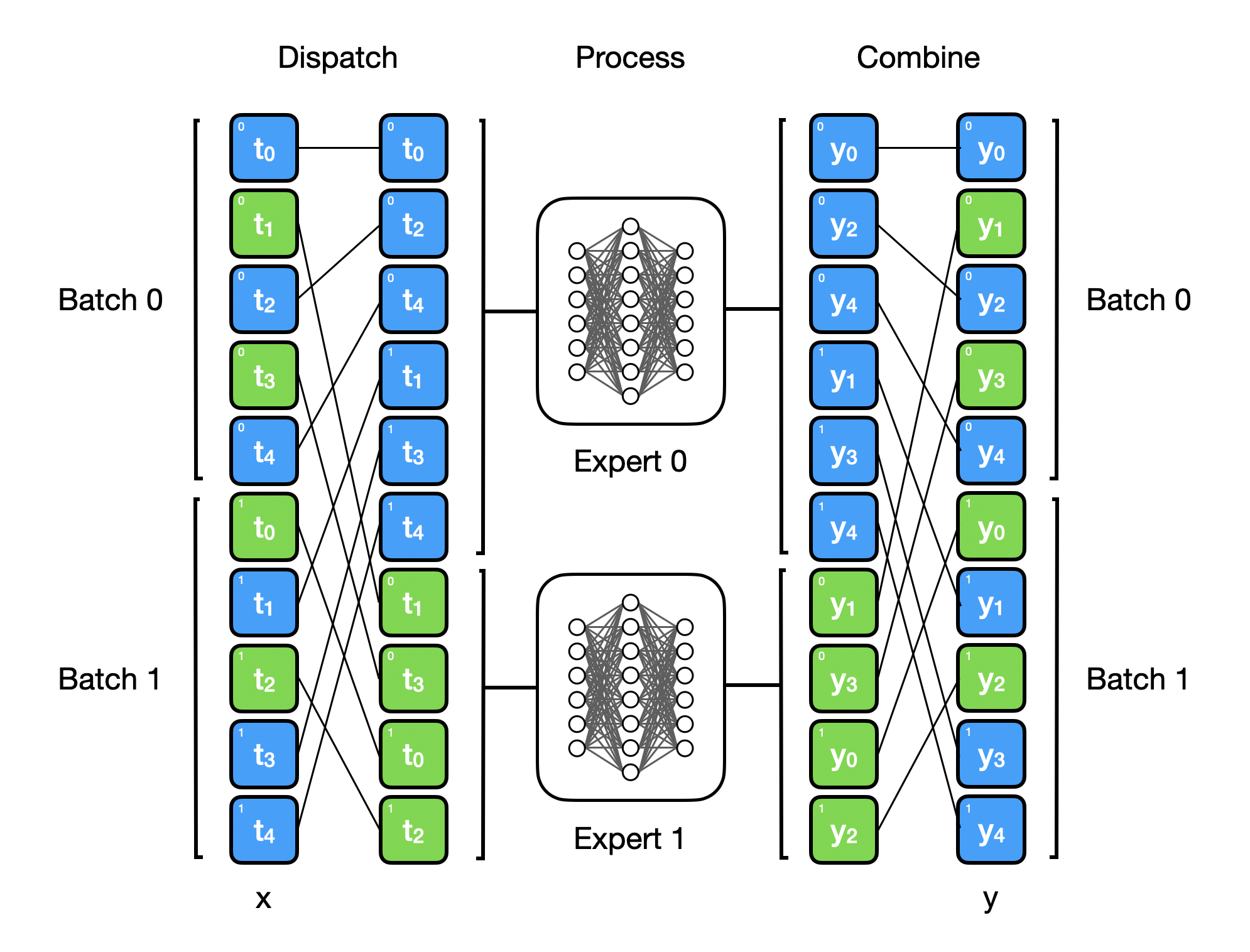
An MoE must:
Dispatch: Filter the input so that only the tokens assigned to "Expert 1" are sent to Expert 1's FFN.
# Get the tokens allocated to each expert
mask_e0 = top1_idx == 0
mask_e1 = top1_idx == 1

x_e0 = x_flat[mask_e0]  # tokens routed to Expert 0
x_e1 = x_flat[mask_e1]  # tokens routed to Expert 1

x_e0 = tensor([
    [ 0.2, -0.1,  0.0,  0.4,  0.1, -0.3,  0.5,  0.2],  # idx 0
    [ 0.5,  0.2, -0.4,  0.0,  0.3,  0.1, -0.2,  0.2],  # idx 2
    [ 0.3, -0.2,  0.1,  0.5, -0.1,  0.0,  0.2,  0.3],  # idx 4
    [-0.3,  0.2,  0.1,  0.0,  0.2, -0.1,  0.3,  0.4],  # idx 6
    [ 0.2, -0.4,  0.3,  0.1,  0.0,  0.2, -0.2,  0.5],  # idx 8
    [ 0.0,  0.2, -0.1,  0.4,  0.3, -0.3,  0.1,  0.2],  # idx 9
], dtype=torch.float32)

x_e1 = tensor([
    [ 0.0,  0.3,  0.2,  0.1, -0.2,  0.4,  0.1, -0.1],  # idx 1
    [-0.1,  0.1,  0.3,  0.2,  0.0, -0.2,  0.4,  0.1],  # idx 3
    [ 0.1,  0.0, -0.2,  0.3,  0.4,  0.2, -0.1,  0.0],  # idx 5
    [ 0.4,  0.1,  0.0, -0.2,  0.1,  0.3,  0.2, -0.1],  # idx 7
], dtype=torch.float32)
Process: Run each token through their assigned expert's FFN.
# Each expert is a FFN, feed the tokens to each expert

class Expert(nn.Module):
    def __init__(self, d_model: int, hidden_dim: int) -> None:
        super().__init__()
        self.net = nn.Sequential(
            nn.Linear(d_model, hidden_dim),
            nn.GELU(),
            nn.Linear(hidden_dim, d_model),
        )

    def forward(self, x: torch.Tensor) -> torch.Tensor:
        return self.net(x)

experts = nn.ModuleList(
    [Expert(d_model=d_model, hidden_dim=hidden_dim) for _ in range(num_experts)]
)

y_e0 = experts[0](x_e0)
y_e1 = experts[1](x_e1)

# Example output (values will differ each run due to random init):
y_e0 = tensor([
    [ 0.09, -0.18,  0.04,  0.13, -0.02,  0.07, -0.11,  0.05],
    [ 0.12, -0.09, -0.03,  0.08,  0.01,  0.10, -0.06,  0.02],
    [ 0.10, -0.16,  0.01,  0.15, -0.04,  0.06, -0.09,  0.04],
    [ 0.05, -0.12,  0.06,  0.11, -0.01,  0.03, -0.08,  0.07],
    [ 0.07, -0.14,  0.09,  0.06,  0.02,  0.04, -0.05,  0.03],
    [ 0.08, -0.10, -0.01,  0.14,  0.00,  0.09, -0.07,  0.01],
], dtype=torch.float32)

y_e1 = tensor([
    [-0.03,  0.11,  0.07, -0.08,  0.05, -0.02,  0.09, -0.01],
    [-0.05,  0.08,  0.10, -0.06,  0.02, -0.04,  0.07,  0.00],
    [-0.01,  0.06,  0.04, -0.10,  0.08, -0.01,  0.05, -0.03],
    [-0.02,  0.09,  0.05, -0.07,  0.03, -0.03,  0.08, -0.02],
], dtype=torch.float32)
Combine: Reassemble the results. If the 1st, 3rd, 5th and 7th tokens were sent to Expert 1, I have to make sure their processed versions end up back at indices 1, 3, 5 and 7 so the sequence structure isn't scrambled.
# Reassemble outputs at original token indices
out_flat = torch.zeros_like(x_flat)

out_flat = tensor([
    [ 0.00,  0.00,  0.00,  0.00,  0.00,  0.00,  0.00,  0.00],
    [ 0.00,  0.00,  0.00,  0.00,  0.00,  0.00,  0.00,  0.00],
    [ 0.00,  0.00,  0.00,  0.00,  0.00,  0.00,  0.00,  0.00],
    [ 0.00,  0.00,  0.00,  0.00,  0.00,  0.00,  0.00,  0.00],
    [ 0.00,  0.00,  0.00,  0.00,  0.00,  0.00,  0.00,  0.00],
    [ 0.00,  0.00,  0.00,  0.00,  0.00,  0.00,  0.00,  0.00],
    [ 0.00,  0.00,  0.00,  0.00,  0.00,  0.00,  0.00,  0.00],
    [ 0.00,  0.00,  0.00,  0.00,  0.00,  0.00,  0.00,  0.00],
    [ 0.00,  0.00,  0.00,  0.00,  0.00,  0.00,  0.00,  0.00],
    [ 0.00,  0.00,  0.00,  0.00,  0.00,  0.00,  0.00,  0.00],
], dtype=torch.float32)

out_flat[mask_e0] = y_e0
out_flat[mask_e1] = y_e1

out_flat = tensor([
    [ 0.09, -0.18,  0.04,  0.13, -0.02,  0.07, -0.11,  0.05],  # idx 0 (e0)
    [-0.03,  0.11,  0.07, -0.08,  0.05, -0.02,  0.09, -0.01],  # idx 1 (e1)
    [ 0.12, -0.09, -0.03,  0.08,  0.01,  0.10, -0.06,  0.02],  # idx 2 (e0)
    [-0.05,  0.08,  0.10, -0.06,  0.02, -0.04,  0.07,  0.00],  # idx 3 (e1)
    [ 0.10, -0.16,  0.01,  0.15, -0.04,  0.06, -0.09,  0.04],  # idx 4 (e0)
    [-0.01,  0.06,  0.04, -0.10,  0.08, -0.01,  0.05, -0.03],  # idx 5 (e1)
    [ 0.05, -0.12,  0.06,  0.11, -0.01,  0.03, -0.08,  0.07],  # idx 6 (e0)
    [-0.02,  0.09,  0.05, -0.07,  0.03, -0.03,  0.08, -0.02],  # idx 7 (e1)
    [ 0.07, -0.14,  0.09,  0.06,  0.02,  0.04, -0.05,  0.03],  # idx 8 (e0)
    [ 0.08, -0.10, -0.01,  0.14,  0.00,  0.09, -0.07,  0.01],  # idx 9 (e0)
], dtype=torch.float32)

# Restore original shape [B, T, D]
out = out_flat.view(2, 5, 8)

out = tensor([
    [  # batch 0
        [ 0.09, -0.18,  0.04,  0.13, -0.02,  0.07, -0.11,  0.05],
        [-0.03,  0.11,  0.07, -0.08,  0.05, -0.02,  0.09, -0.01],
        [ 0.12, -0.09, -0.03,  0.08,  0.01,  0.10, -0.06,  0.02],
        [-0.05,  0.08,  0.10, -0.06,  0.02, -0.04,  0.07,  0.00],
        [ 0.10, -0.16,  0.01,  0.15, -0.04,  0.06, -0.09,  0.04],
    ],
    [  # batch 1
        [-0.01,  0.06,  0.04, -0.10,  0.08, -0.01,  0.05, -0.03],
        [ 0.05, -0.12,  0.06,  0.11, -0.01,  0.03, -0.08,  0.07],
        [-0.02,  0.09,  0.05, -0.07,  0.03, -0.03,  0.08, -0.02],
        [ 0.07, -0.14,  0.09,  0.06,  0.02,  0.04, -0.05,  0.03],
        [ 0.08, -0.10, -0.01,  0.14,  0.00,  0.09, -0.07,  0.01],
    ],
], dtype=torch.float32)
4. The Auxiliary Loss (Load Balancing)
Which experts the router favours at the start is random and down to the initialisation of the router weights.
At the start of training, a router could randomly favour an expert giving it more updates. That expert therefore gets "smarter", so the router sends it even more tokens. Eventually, any other experts could be ignored entirely.
To handle this, I add a small auxiliary loss term that penalises the router if it isn't distributing tokens roughly equally across all experts.
# Fraction of tokens sent to each expert
expert_counts = torch.bincount(top1_idx, minlength=2).float()
expert_counts = tensor([6, 4])

tokens_per_expert = expert_counts / expert_counts.sum().clamp_min(1.0)
tokens_per_expert = tensor([0.6, 0.4])

# Mean router probability per expert
mean_router_prob = probs.mean(dim=0)
mean_router_prob = tensor([0.5120, 0.4880])

# Switch-style auxiliary loss
aux_loss = 2 * torch.sum(tokens_per_expert * mean_router_prob)
aux_loss = 1.0048   # 2 * (0.6 * 0.5120 + 0.4 * 0.4880)
This follows the auxiliary loss formulation from the Switch Transformer (Fedus et al., 2021).
What I am skipping (The "Minimal" Caveats)
This is a minimal MoE block implementation and there are things I'm skipping. For instance:
- Capacity Factor: production models cap how many tokens each expert processes per batch. When an expert's buffer is full, overflow tokens are dropped entirely - skipped on that forward pass. Without this, a skewed router can crash the GPU with memory overflows.
- Expert Parallelism: I'm not doing anything smart with compute like splitting experts across different GPUs; everything runs on one device.
- Top-k Case, k > 1: I'm not exploring the general top-k case.
- Router Noise: many MoEs add noise to the router to help it explore different experts during training.
Building An MoE From Scratch
With the mechanics of routing and dispatching laid out, I can now assemble the full model. For this I'm building a Decoder-only transformer (similar to the GPT family) in PyTorch - not every primitive, but every MoE-specific component.
This is the full model architecture:
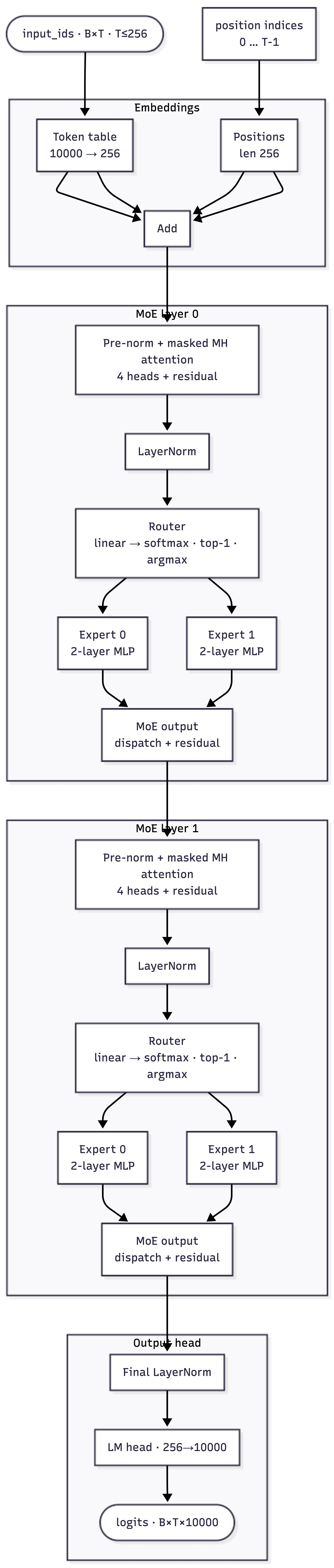
In my decoder, the MoE layer replaces the standard Feedforward Network in every block. Each block now consists of a masked Self-Attention layer followed by my sparse MoE layer.
The full MoE Layer:
class MoELayer(nn.Module):
    def __init__(
        self,
        d_model: int,
        hidden_dim: int,
        num_experts: int,
    ) -> None:
        super().__init__()
        self.num_experts = num_experts
        self.router = Router(d_model=d_model, num_experts=num_experts)
        self.experts = nn.ModuleList(
            [Expert(d_model=d_model, hidden_dim=hidden_dim) for _ in range(num_experts)]
        )
        self.last_aux_loss = torch.tensor(0.0)
        self.last_routing_stats: dict[str, torch.Tensor] = {}

    def forward(self, x: torch.Tensor) -> torch.Tensor:
        batch_size, seq_len, d_model = x.shape
        # Flatten [B,T,D] -> [B*T,D] so router picks an expert per token (no token mixing)
        x_flat = x.reshape(batch_size * seq_len, d_model)
        probs, top1_idx = self.router(x_flat)

        # Simple top-1 dispatch and recombine to original token order
        out_flat = torch.zeros_like(x_flat)
        expert_counts = torch.bincount(top1_idx, minlength=self.num_experts).float()
        for expert_id, expert in enumerate(self.experts):
            token_mask = top1_idx == expert_id
            if token_mask.any():
                # Dispatch this expert's tokens, run expert MLP, recombine to matching token rows
                out_flat[token_mask] = expert(x_flat[token_mask])

        # Load-balancing loss (Switch-style): penalise skewed routing
        tokens_per_expert = expert_counts / expert_counts.sum().clamp_min(1.0)
        mean_router_prob = probs.mean(dim=0)
        aux_loss = self.num_experts * torch.sum(tokens_per_expert * mean_router_prob)     # returned separately at class level

        return out_flat.view(batch_size, seq_len, d_model)
Here is the full router (note it's just a single linear layer):
class Router(nn.Module):
    def __init__(self, d_model: int, num_experts: int) -> None:
        super().__init__()
        self.num_experts = num_experts
        self.proj = nn.Linear(d_model, num_experts)

    def forward(self, x_flat: torch.Tensor) -> tuple[torch.Tensor, torch.Tensor]:
        logits = self.proj(x_flat)
        probs = torch.softmax(logits, dim=-1)
        # Hard top-1 routing: choose one highest-probability expert per token
        top1_idx = torch.argmax(probs, dim=-1)
        return probs, top1_idx
Here is the full expert (this is just a simple FFN, which is exactly what the MoE layer replaces):
class Expert(nn.Module):
    def __init__(self, d_model: int, hidden_dim: int) -> None:
        super().__init__()
        self.net = nn.Sequential(
            nn.Linear(d_model, hidden_dim),
            nn.GELU(),
            nn.Linear(hidden_dim, d_model),
        )

    def forward(self, x: torch.Tensor) -> torch.Tensor:
        return self.net(x)
Training The Model
Data
To see if my from scratch MoE actually learns, I used the TinyStories dataset. It fits well because it contains short, simple stories with a limited vocabulary, allowing me to see meaningful results without needing to hire double-digit H200s.
One day, a little girl named Lily found a needle in her room. She knew it was difficult to play with it because it was sharp. Lily wanted to share the needle with her mom, so she could ...

Once upon a time, there was a little car named Beep. Beep loved to go fast and play in the sun. Beep was a healthy car because he always had good fuel. Good fuel made Beep happy and strong. One day ...

One day, a little fish named Fin was swimming near the shore. He saw a big crab and wanted to be friends. "Hi, I am Fin. Do you want to play?" asked the little fish. The crab looked at Fin and said ...
I downloaded this from Hugging Face, roneneldan/TinyStories.
Data Pipeline
TinyStories comes as a training set containing 2.12 million short stories and a validation set of 22k stories. I set the validation set aside as my test set and took the full training set and carved out a 5% dev split for validation.
| Split | Stories |
|---|---|
| Train | 2,013,733 |
| Dev | 105,986 |
| Test | 21,990 |
I trained a custom BPE tokeniser (vocab size 10,000) on the training split to avoid data leakage.
Story tokenised: ['One', 'day', ',', 'a', 'little', 'girl', 'named', 'Lily', ...]
Story as tokens: [383, 252, 15, 155, 295, 342, 397, 254, ...]
In the training set every story is appended with an <EOS> token and concatenated into a massive 1D token stream.
During a training run, a random 256 token window is sampled from the token stream. The model is constantly tasked with predicting the next token in these slices.
The Model at a Glance
I started by training a small model with 2 experts per layer, a model dimension of 256 and a context length of 256 tokens.
This totals ~7.8 million parameters, but because of the sparse routing, only ~6.7 million are active during any single forward pass.
Loss
I trained the model using the standard language modelling objective: minimising next-token cross-entropy.
ce_loss = torch.nn.functional.cross_entropy(logits, targets)
CE loss, however, only rewards accuracy - not balance across experts. Routers will learn to pick one expert and stop there. The auxiliary loss defined earlier prevents this.
To control this I add a small coefficient, load_balance_coef, to scale it - a gentle nudge, not a shove.
Too low (0.0) and one expert dominates; too high (0.1) and the model sacrifices accuracy for balance. 0.01 keeps all experts active without
distracting the model from its primary job: next-token prediction.
total_loss = ce_loss + load_balance_coef * aux_loss
Optimisation
I used AdamW - standard for transformers, since it handles the complex, high-dimensional landscapes of LLM training more reliably than typical gradient descent.
optimizer = torch.optim.AdamW(
    model.parameters(),
    lr=0.0003,
    weight_decay=0.1
)
The Training Run
I trained for 10,000 steps and it worked! I ran this on my MacBook Pro (M1 Pro) using the mps backend and it took 1 hour and 20 minutes to train. These 10,000 steps covered ~37% of the training data, plenty of stories for the model to start learning.
Here are some example outputs from the trained model continuing the story "Once upon a time":
Once upon a time, there was a little boy named Timmy. Timmy loved to play outside in the sunshine. One day, Timmy's mom told him to go outside and play outside. Timmy went to the park and Timmy saw a big, red ball. He wanted to play with ...

Once upon a time, there was a little girl named Lily. Lily loved her mommy and daddy very much. She had the prettiest dress and wore a pink dress, her face. One day, Lily's mommy gave her some love and they went for a walk. Lily saw Mr Jones and said, "Mommy, can I please?" ...

Once upon a time, there was a little girl named Lily. She loved to skip and sing for her family. One day, Lily was feeling a little sad because she couldn't find her mommy. She asked her mommy if she could go home, but her mommy told her to stay close to her. ...
These use temperature = 0.8 and top_k = 50. Not perfect, but pretty good for a small, untuned, local model.
Performance
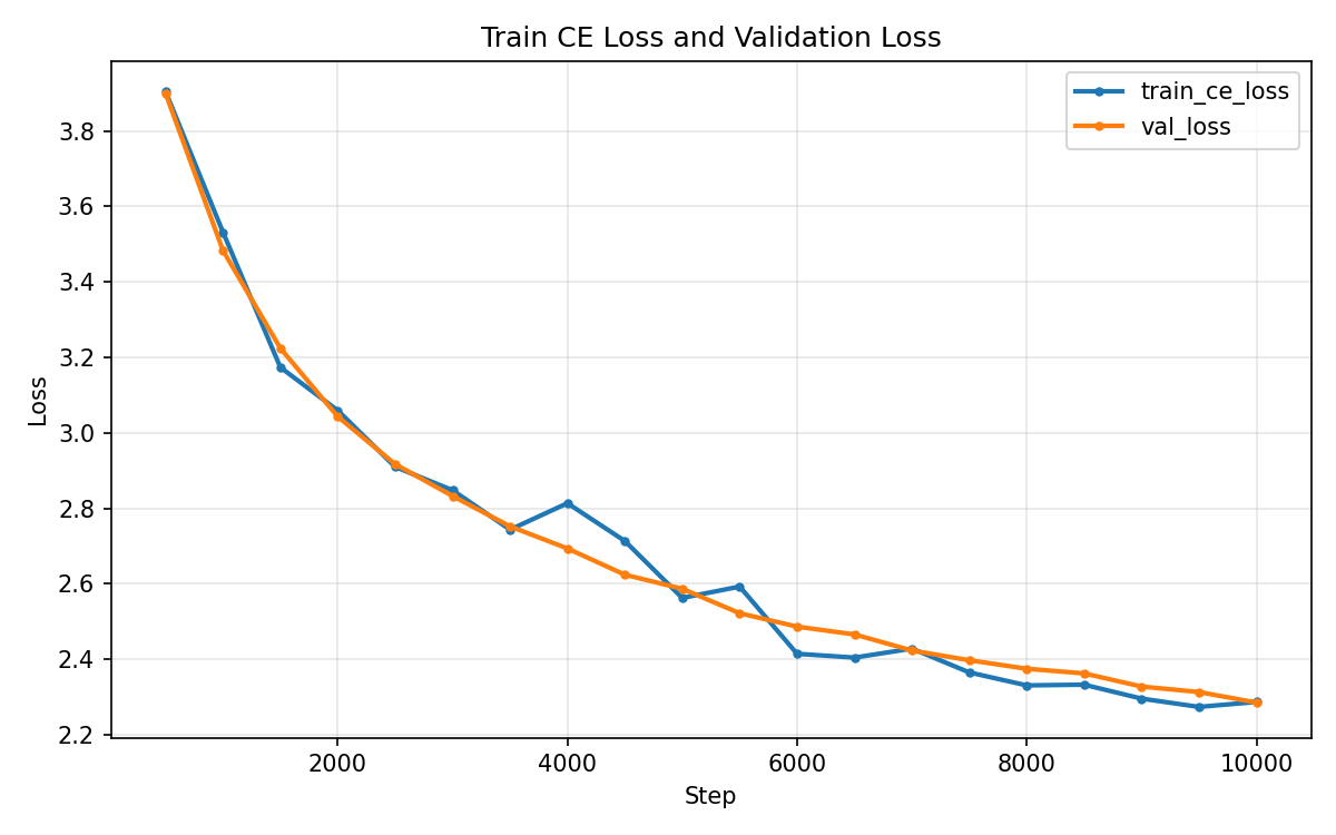
First let's look at the primary objective - cross-entropy loss. I want a smooth downward trend for both the training and validation sets. This would show the model is learning well (and it does!).
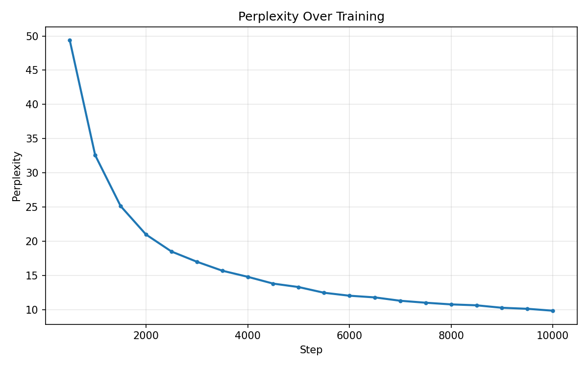
While loss is what I'm optimising, perplexity tells me how "confused" the model is. It represents the number of likely options the model is considering for the next token. Seeing this drop rapidly at the start of training shows the model is quickly picking up the basic structure of English, e.g., knowing that "Once" is usually followed by "upon a time".
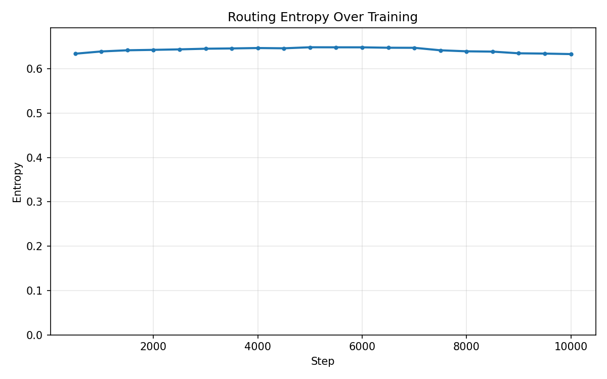
This is where things get interesting. Routing entropy measures the diversity of the Router's decisions. For a system with 2 experts, the maximum entropy is ~0.69 (ln(2)). If the entropy is near this peak, the router is utilising both experts equally. If it drops towards zero, the router has collapsed onto a single expert.
My model stays level at just over 0.6 - high enough to prove it hasn't collapsed, but just below the maximum, suggesting the router is actually making meaningful, non-random choices.
To really see the "Mixture of Experts" in action, I can look at the expert usage heatmap. Even with just two layers and two experts, this 2x2 grid is telling: it shows the percentage of tokens assigned to each expert at every layer. Near 50/50 means the router isn't picking favourites.
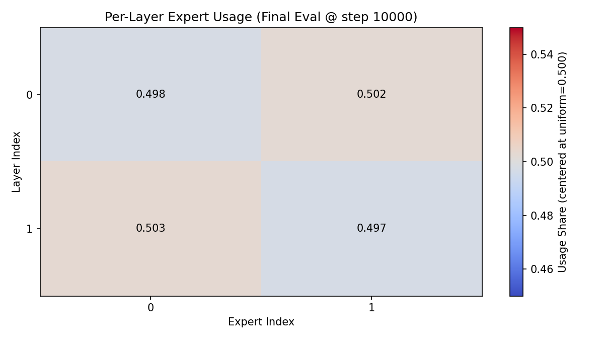
Overall, these metrics confirm a healthy training run: the model converged steadily while maintaining high routing diversity.
Do the Experts Actually Specialise?
The entropy tells me the router is active - but what is it actually routing? I ran a quick analysis over 500 validation samples. Layer 0 is
noisy and hard to read. Layer 1 is more interesting: 76% of token types consistently route to the same expert more than 70% of the time, and
the split is interpretable. Expert 0 claims punctuation, conjunctions and emotional-state adjectives (., ,, and, but, tired,
afraid, grateful); Expert 1 claims past-tense action verbs and concrete physical nouns (had, looked, played, door, window, dragon).
At Layer 1, Expert 0 handles language scaffolding; Expert 1 handles story events.
The Layer 0 vs Layer 1 gap makes sense - transformers tend to build surface features early and semantics later. High-frequency glue words
(it, her, so, went) stay ambiguous across both layers, since their role is too context-dependent to resolve from token identity alone.
Whether this sharpens on more diverse data and at larger scale is the natural next question.
The Comparison: MoE vs Dense (The Reality Check)
To see if the complexity of MoE was worth it, I trained a dense (non-MoE) control model. I replaced every MoE layer with a single, standard FFN of the same size as one of my experts. This gives a fair fight: a traditional transformer approach with fewer total parameters but roughly the same number of active parameters per token.
| Metric | MoE (2 Experts) | Dense (Control) |
|---|---|---|
| Active parameters | 6,766,596 | 6,765,568 |
| Total parameters | 7,817,732 | 6,765,568 |
| Best validation loss | 2.285 | 2.276 |
| Total training time (s) | 4825.0 | 2475.8 |
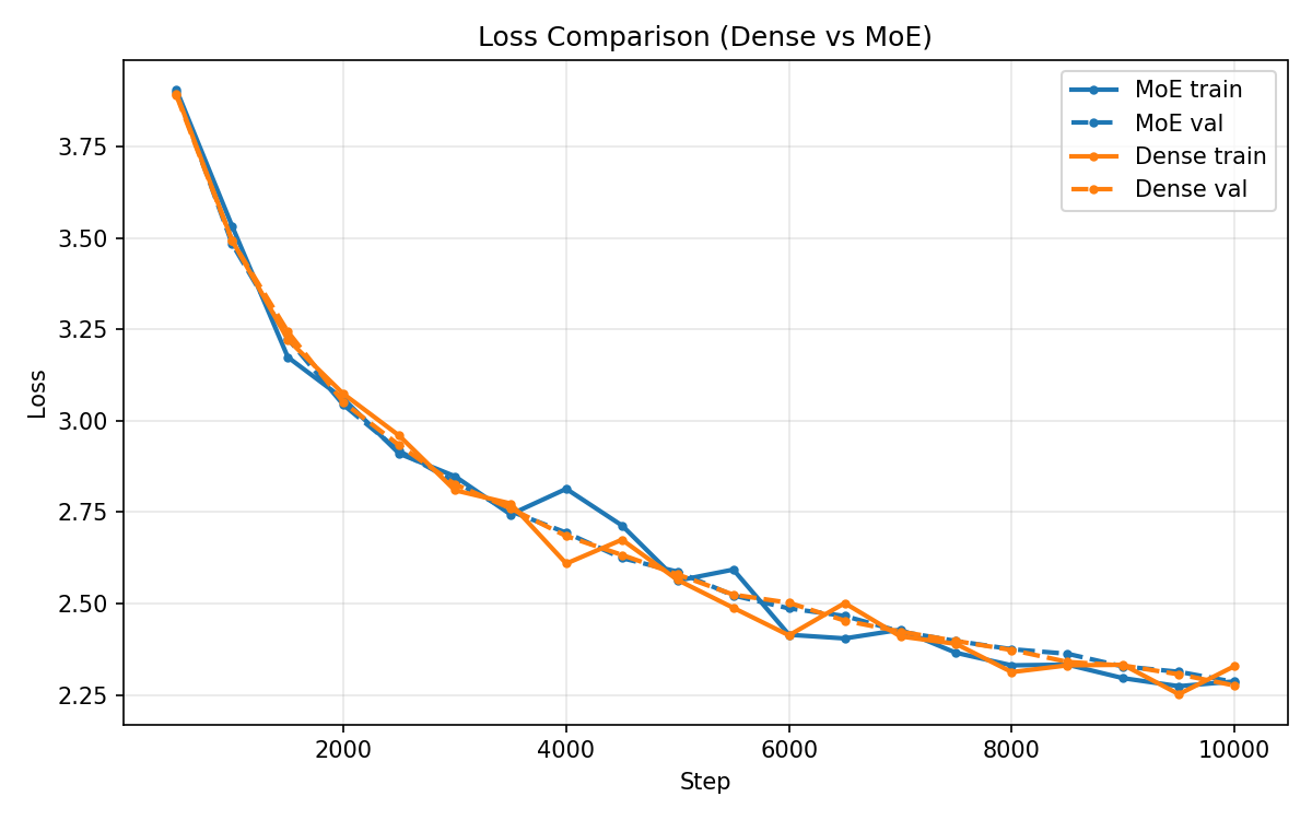
Visibly not much between them - the dense model actually just edges out the MoE in both accuracy and speed. So, MoE is worse then?
At this scale, yes (by a whisker) - but that's exactly what I'd expect. There are a couple of reasons why:
- The Routing Tax: at small scales the router overhead is proportionally expensive. The model spends precious capacity figuring out how to delegate, whereas the dense model can put all its effort into learning the stories. My unoptimised logic makes this worse (hence taking double the time to train) - production implementations use CUDA kernels - but even optimal routing can't overcome the fundamental cost at 7.8M parameters.
- The Scaling Law: MoE is a scaling strategy. Its benefits usually only kick in once you reach hundreds of millions of parameters.
Getting the mechanics right matters more than winning at 7.8M parameters - these are the same building blocks that let DeepSeek and Mixtral scale to trillions.
Next Steps
This basic implementation is just the foundation. To move towards production-grade performance, several levers remain to be pulled:
Capacity Enforcement: In this version, an expert takes every token the router sends it. In real-world systems, a buffer limit is used to prevent one expert from overflowing and crashing the GPU.
Top-2 Routing: Moving beyond Top-1 allows tokens to be processed by two experts and blended. This often leads to smoother training and better knowledge sharing.
Auxiliary-Free Routing: The load_balance_coef feels like an arbitrary dial because it is. Newer approaches ditch the auxiliary loss
entirely, using a per-expert bias term updated based on recent load. Cleaner and one less hyperparameter to tune.
Data Heterogeneity: TinyStories is samey by design. To really see experts specialise (maybe one expert that's better suited for maths or one for creative writing), the next step is mixing in more diverse datasets.
Conclusion & Learnings
This project was never about breaking benchmarks on a single MacBook; it was about peering under the hood of MoE to see how the gears turn - and after 10,000 steps, the MoE generates coherent stories with every expert pulling its weight.
However, the comparison showed that the benefits of MoE only emerge at scale, where the sparse routing overhead becomes negligible against the gains. At this tiny parameter count, the routing tax means a dense model is often more efficient. The true magic of MoE only reveals itself at billions of parameters, where the sparse routing is what makes training and serving at that scale computationally tractable.
The hard part is done. Scaling to 1.6T parameters is left as an exercise for the reader.
Code for this post: moe-from-scratch